Deep Bayesian Generative Models for Classification

Introduction

Here is the question we wish to answer: “How can we leverage generative models with unlabeled data to improve classification accuracy?” Before we jump into the math and code example, I’d like to give an overview of some common dichotomies in machine learning.

Data and Algorithmic Models

Leo Breiman illustrates the dichotomy between Data Models and Algorithmic Models in his paper Statistical Modeling: The Two Cultures. The truths that Breiman unpacked almost 20 years ago still hold true today. Following the conventions laid out in that paper, any reference to a “model” will be a type of algorithmic model, which attempts to predict the response or label $y$ for a given input $x$.

Supervised, Unsupervised, and Semi-Supervised Learning

Supervised and unsupervised learning summarize the extremes of the training regimen spectrum for algorithmic models. Supervised learning equates to training a model with labeled data, while unsupervised learning expects a model to learn useful patterns without labels. Semi-supervised learning falls in between the two, where the model employs labeled and unlabeled data to perform a task.

Discriminative and Generative Models

The architectures of algorithmic models generally fall into two categories: discriminative and generative models. For a supervised learning task, discriminative models learn the mapping between the set of labels ${Y}_j$ and the set of data ${X}_i$; a label prediction $\hat{y}$ is made by applying a datum $x$ to the model, which is acting as a complicated function. On the other hand, generative models first learn a joint distribution of the set of labels ${Y}_j$ and the set of data ${X}_i$; a label prediction $\hat{y}$ is achieved by factoring that joint distribution into a conditional distribution $p(Y|X=x)$ and then sampling from that conditional distribution. If generative models sound more complicated, it’s because they usually are; however, you can use those models for a variety of tasks, even beyond the one that is interesting at the moment.

Bayesians and Frequentists

These differences between generative and discriminative models reflect the differing approaches of the Bayesian and Frequentist schools of thought respectively. Frequentists believe that the parameters of interest are fixed and unchanging under all realistic circumstances; therefore, discriminative models ask, “To which category $y$ does $x$ belong?” Bayesians view the world probabilistically rather than as a set of fixed phenomena that are either known or unknown; therefore, generative models ask, “Which category distribution $p(y)$ is most likely to generate this datum $x$? Both statistical schools of thought have developed ways to validate their models, estimate error and variance, and incorporate pre-existing information, and each has their proponents. But sometimes it just boils down to common sense.

Mathematics

Let’s rephrase the original question into a thesis: We are first going to learn the distribution of data by training a generative model with unlabeled data, and then learn a mapping from the inferred latent distribution to the label categories using labeled data only.

The key difference between this paradigm and the discriminative supervised learning approach is that the mapping learned by a generative model stretches from a distribution of data, not just the data points themselves. Intuitively, mapping from a distribution will allow us to generalize better to unseen data points in our classification task. To be fair, discriminative models can achieve a similar effect by adding noise to the input data, but the math is less flexible than the Bayesian formulation.

In order to learn the distribution of data, we will need to introduce a few mathematical concepts: the variational lower bound, Kulback Liebler divergence, and the reparameterization trick.

Variational Lower Bound

Michael Jordan (the statistician) is credited with formalizing variational bayesian inference in An Introduction to Variational Methods for Graphical Models. We will unpack section 6 of that paper in detail with the following derivation of the variational lower bound, or the ELBO:

\[\begin{align*} \tag{1} \log p(X) &= log \int_Z p(X,Z) \\ \tag{2} &= \log \int_Z p(X,Z) \frac{q(Z)}{q(Z)} \\ \tag{3} &= \log \Bigg ( \mathbb{E}_q \bigg [ \frac{p(X,Z)}{q(Z)} \bigg ] \Bigg ) \\ \tag{4} &\geq \mathbb{E}_q \bigg [ \log \frac{p(X,Z)}{q(Z)} \bigg ] \\ \tag{5} &= \mathbb{E}_q \big [ \log p(X,Z) \big ] - \mathbb{E}_q \big [ \log q(Z) \big ] \\ \tag{6} &= \mathbb{E}_q \big [ \log p(X,Z) \big ] + H[Z] \\ \end{align*}\]

We start with a definition of marginal probability.
Here we introduce q(Z); this distribution will approximate the true posterior p(Z|X). q(Z) belongs to a variational family of distributions selected to make its inference more computationally tractable. We will cover the details of this inference in a later section.
We apply the definition of expectation.
We apply Jensen’s Inequality, which is best understood graphically.
We apply a property of logarithms.
We define H[Z] to be Shannon’s Entropy.

We now have a lower bound, $L$, on the data likelihood, which we want to maximize!

Kulback Lieber Divergence

Let’s rewrite this lower bound and apply the KL Divergence definition:

\[\begin{align*} \tag{1} L &= \mathbb{E}_q \bigg [ \log \frac{p(X,Z)}{q(Z)} \bigg ] \\ \tag{2} L &= \mathbb{E}_q \bigg [ \log \frac{p(Z|X)p(X)}{q(Z)} \bigg ] \\ \tag{3} L &= \mathbb{E}_q \bigg [ \log \frac{p(Z|X)}{q(Z)} \bigg ] + \mathbb{E}_q \bigg [ \log p(X) \bigg ] \\ \tag{4} L &= -\mathbb{E}_q \bigg [ \log \frac{q(Z)}{p(Z|X)} \bigg ] + \log p(X) \mathbb{E}_q \bigg [1 \bigg ] \\ \tag{5} L &= -D_{KL} \bigg ( q(Z) || p(Z|X) \bigg ) + \log p(X) \\ \end{align*}\]

So in order to maximize $L$, we must minimize the divergence between our true posterior, $Z$, and our approximation, $q(Z)$. Naively differentiating and optimizing this lower bound results results in high-variance sampling. Which is why we need a trick!

Backpropagation and the Reparameterization Trick

The beauty of Auto-Encoding Variational Bayes is the blending of the variational approach with neural networks and backpropagation. Classically, variational inference has been the method for transforming a Bayesian sampling framework into an optimization problem, with new applications all the time. Kingma et al extend that classical application with the reparameterization trick in order to allow backpropagation to pass through the stochastic processes of the model, specifically the $Z$ variables in the above section. The trick involves factorizing the sampling distribution into parameters that are inferred and noise that is injected into the model. Using a Normal distribution as an example:

\[\begin{align*} z &\sim Q(Z) = \mathcal{N}(\mu, \sigma^2) \\ z &= \mu + \sigma \odot \epsilon, \epsilon \sim \mathcal{N}(0, 1) \\ \end{align*}\]

Variational Autoencoder

Kingma et al present a simple example of the Variational Autoencoder (VAE) in Appendix B of Auto-Encoding Variational Bayes that we will unpack here. $p(Z|X)$ is modeled a neural network where $Z = \mu + \sigma \odot \epsilon, \epsilon \sim \mathcal{N}(0, I)$. Draws from $Z$ serve as Gaussian inputs to the generative model, $q(X|Z)$, which generates reconstructions of the inputs.

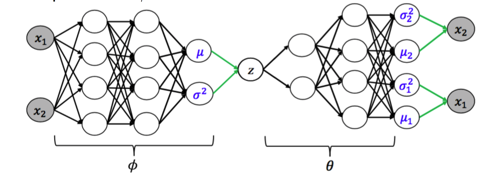
A three layer Variational Autoencoder with a Gaussian posterior and generative model.

The variational lower bound for this model that we must maximize is (note that we condition on $X$ now unlike the previous section):

\[\begin{align*} \tag{1} L &= -D_{KL} \bigg ( q(Z) || p(Z|X) \bigg ) + \log p(X | Z) \\ \tag{1} L &\approx \frac{1}{2} \sum_{j=1}^J \bigg ( 1 + \log \big ((\sigma_j)^2 - (\mu_j)^2 - (\sigma_j)^2 \big ) \bigg ) + \frac{1}{S} \sum_{s=1}^S \log p(X|Z^{(s)}) \\ \end{align*}\]

$J$ is the dimension of the latent variable $Z$, and $S$ is the number of samples that are passed into the generative model before calculating the log likelihood of the input data, $X$, under the parameters inferred by the generative model.

The first term can be viewed as a regularizing term, which forces $Z$ to be close to the prior, and the log likelihood term can be viewed as a reconstruction term (autoencoder parlance), where the generated data must be close to the input data.

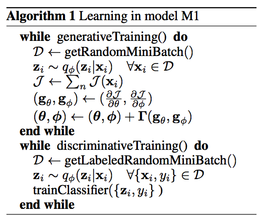
Semi-Supervised Learning with Deep Generative Models

In the original VAE paper, the authors employ the generative model to reconstruct image inputs so as to show that the algorithm learns a set of meaningful latent variables $Z$. In Semi-Supervised Learning with Deep Generative Models, Kingma et al use the VAE framework as a preprocessing step before discriminative training:

First train the VAE using unlabeled data, then train the classifer on top of the VAE.

Implementation

The Jupyter Notebook for this section can be found here.

A classic binary classification dataset is the Wisconsin Breast Cancer Diagnostic dataset. It contains 569 samples with 30 variables each; each sample is labeled as “benign” or “malignant”. Sklearn makes it easy to import the data. Our goal is to build a semi-supervised model that leverages unlabeled data for the purposes of increasing classification accuracy.

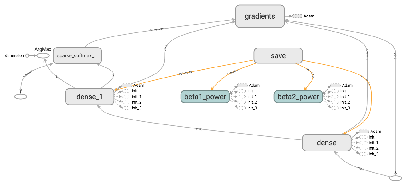
First, we build an straightforward two layer neural network, visualized with Tensorboard:

Supervised Graph

Here’s the training loss curve:

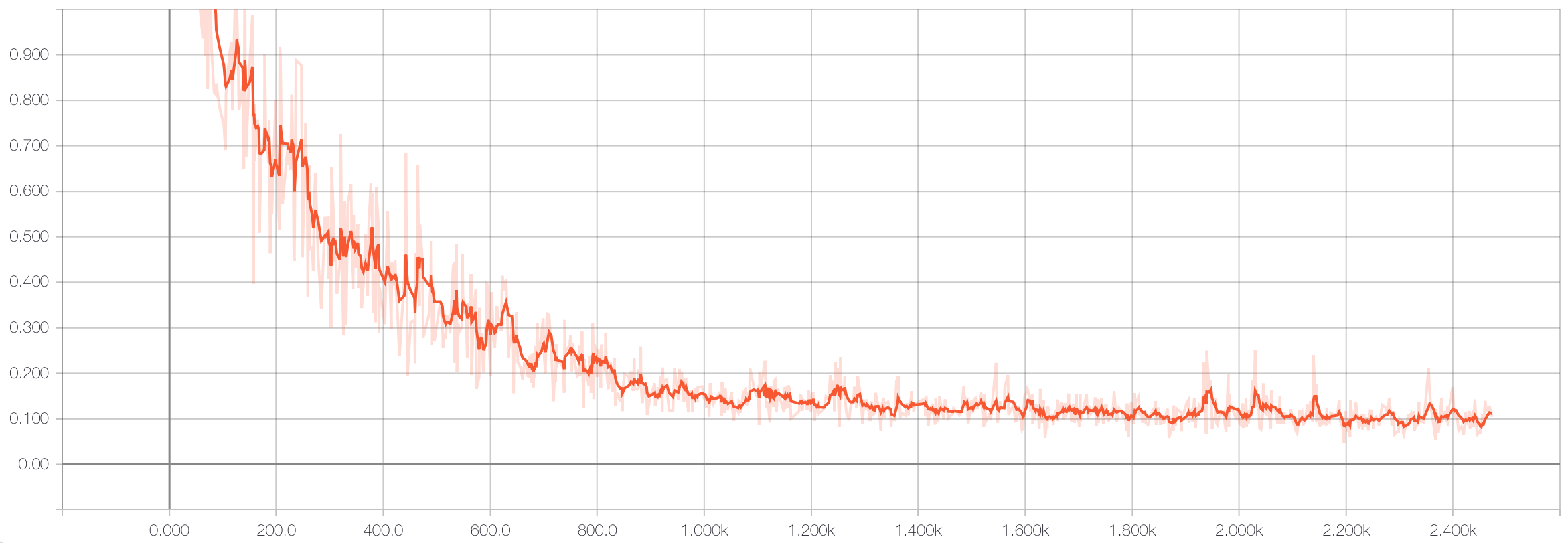
Training Loss for Supervised Graph

Which results in an accuracy on the hold-out test set of 98.6%. Very nice!

Next, we build a two layer VAE with a linear neural network build on top of $Z$. Here’ s the Tensorboard visualization:

Semi-Supervised Graph

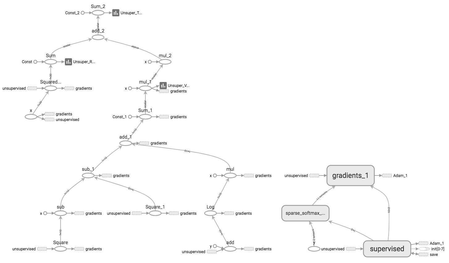
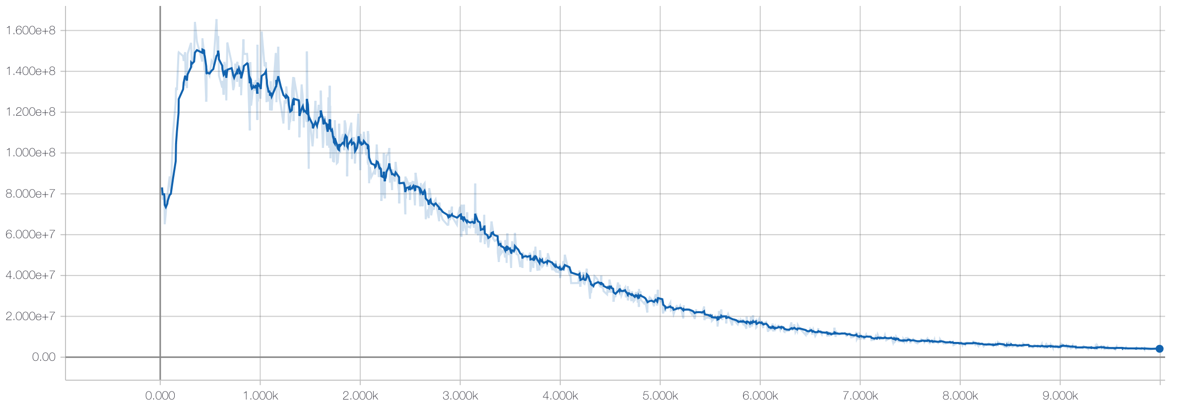
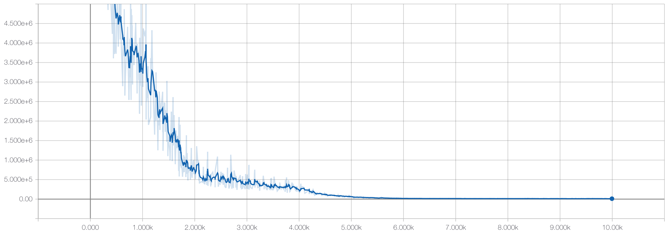
We then train the autoencoder portion of the model on the training data without utilizing the labels:

VAE Loss

Reconstruction Loss

Then we freeze the weights on the autoencoder portion and only train the weights of the linear model with the labeled training data:

Linear Model Loss

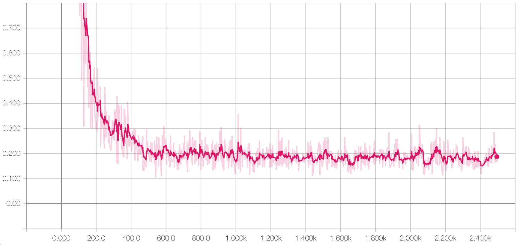
Which results in an accuracy on the hold-out test set of 98.6%. Which matches the results from the supervised model! Why is this exciting?

Conclusion

This pair of results show that the VAE has learned a set of features $Z$ that could be linearly separated to achieve the same accuracy as a non-linear neural network with many more variables. This size of this dataset and the absence of truly unlabeled data limits our ability to go further, but real world classification problems that fit the problem description abound, simply because labeling data is almost always more expensive than obtaining lots of unlabeled data.