2017 NBA Hackathon Questions

The application to the 2017 NBA Hackathon featured several interesting questions, two of which I would like to unpack in this post:

1. How likely is a team to lose consecutive games in an 82-game season?
2. How much money is the NBA likely to generate from playoff ticket sales?

All of the R code for both questions can viewed in this repo.

Probability of Consecutive Losses

Imagine that the Warriors have a $80$% of winning each game during their 82-game regular season. What’s the chance they don’t lose back-to-back games? This was a popular question after Kevin Durant joined the Warriors before the 2016-2017 season.

Approximation Approach

Monte Carlo simulations are a simple method to approximate probability distributions; once you have an approximation of a distribution, generating a point estimate, such as an expected value, is straight forward. The plot below shows the first $10000$ samples from such a simulation, which will eventually converge to the expected value of the distribution.

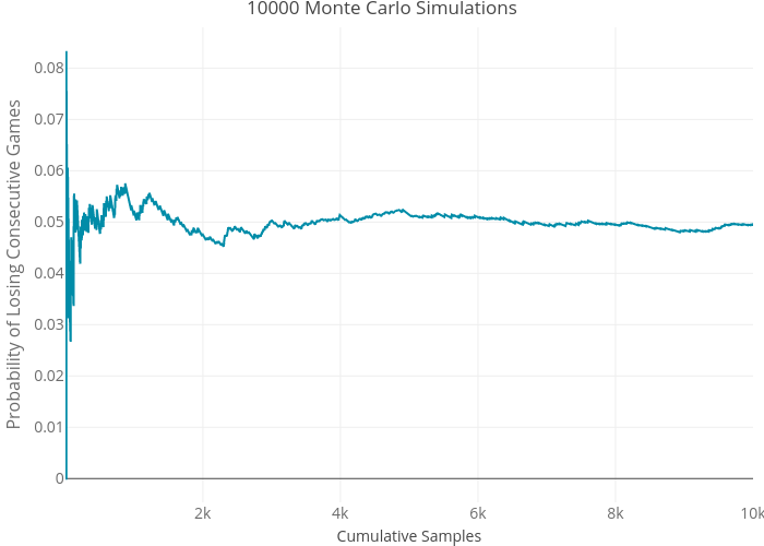
The simulation predicts that the Warriors have a $\underline{5.041\%}$ chance of not losing consecutive games (code). It would would be helpful to know the precision of this approximation. The variance of an expected value from a Monte Carlo simulation, with samples ${\phi_1, …, \phi_n}$, is described by:

We can compute $\text{Var}[\phi]$ since our samples are drawn from a Binomial distribution

With $200000$ samples, $Var_{MC}[\overline{\phi}] = 6.56 \times 10^{-5}$, which means we can expect the true value to be contained within the following interval for 95% of all MC simulations:

Now let’s calculate the exact answer and see how our approximation compares.

Exact Approach

Let’s consider three distinct groups of games and their total counts for the Warriors 82-game season, where $l$ represents the number of losses:

• losses that are followed by a win (LW), of which there are $(l - 1)$ but represent $2(l-1)$ games.
• a season-ending loss (L), of which there is $1$.
• single, standalone wins (W), of which there are $82 - 2(l - 1) - 1 = 83 - 2l$.

We arrive at the total number of units by adding all three groups together: $83 - 2l + (l - 1) + 1 = 83 - l$. These three groups can be placed in any order and the season can be guaranteed to not contained any back-to-back losses. We just need to figure out how to enumerate these combinations.

If we could lump two of the units together, we would be choosing the ordering of two groups and could use the binomial formula; and lucky for us, we can do just that! If we group the two types of units with losses together (of which there are $l$), we don’t have to designate which loss is the season-ending one. With this insight, we have $83-l$ total slots to put a loss, and have $l$ losses to place, which gives us the following equation for the number of $l$-loss seasons that do not contain consecutive losses:

If we consider the Warriors probability of winning a game is 80%, and we want to get the total probability over all possible seasons, we get the following equation:

So the Warriors had exactly a $\underline{5.88}$% chance of not losing consecutive games if indeed they had an 80% chance of winning every game. And the exact answer falls within the range given by our Monte Carlo simulation; yes, all is right with the world. If we wanted to make this problem more interesting, we could take into account the Warriors schedule and calculate the win probability of each game. But now it’s time to talk about cash flow!

Expected Playoff Gate Revenue

How much money from ticket sales can the NBA expect to bring in during the Playoffs? The League provided two datasets as a part of the Hackathon application:

1. The win probabilities for home and away games for every combination of teams (view data).
2. The expected gate revenue at each NBA stadium for all four playoff rounds (view data).

First, we need to figure out the expected revenue from each matchup, and this is dependent on how many games are played of the 7-game series.

7-Game Series Math

Let’s start simply by considering the probabilities that a 7-game series ends in either $N = {4,5,6,7}$ games if the two teams have equal probabilities of winning:

• N = 4. $2 \binom{3}{3} / 2^3 = 0.125$
• N = 5. $2 \binom{4}{3} / 2^4 =0.25$
• N = 6. $2 \binom{5}{3} / 2^5 = 0.3125$
• N = 7. $2 \binom{6}{3} / 2^6 = 0.3125$

Notice how these four numbers sum to $1$, which confirms that we are working with a valid probability distribution. In this equations above, the denominator gives the total number of possible win/loss combinations and the numerator describes the number of outcomes in which 4 games is won by either team (hence the doubling factor in the numerator).

Now let’s make the problem more complex: we expect one team (Warriors) to beat the other team (Spurs) with probability $p = 0.55$. Now we have to split up the probability of the Warriors winning and the Spurs winning:

• N = 4. $\binom{3}{3} (p^4 + (1-p)^4) = 0.133$
• N = 5. $\binom{4}{3} (p^4(1-p) + (1-p)^4p) = 0.255$
• N = 6. $\binom{5}{3} (p^4(1-p)^2 + (1-p)^4p^2) = 0.309$
• N = 7. $\binom{6}{3} (p^4(1-p)^3 + (1-p)^4p^3) = 0.303$

These calculations show that the more lopsided a matchup, the more likely the series is to last fewer games! But we can still make the problem more complicated by taking into account home and away games; for this discussion, we will assume the 2-2-1-1-1 playoff series format. If we assume that the Warriors have a $p_h$ chance of winning at home against the Spurs and a $p_a$ chance of winning away against the Spurs, then the following expressions describe the probability that the series ends in $N$ games:

N = 4, 2 Home games, 2 Away games.

\(p_h^2p_a^2 + (1-p_h)^2(1-p_a)^2\)

N = 5, 3 Home games, 2 Away games.

\(\begin{align} \binom{2}{1} &\left[ p_h^2p_a^2(1-p_h) + (1-p_h)^2(1-p_a)^2p_h\right] +\\\\ \binom{2}{1} &\left[ p_h^3p_a(1-p_a) + (1-p_h)^3(1-p_a)p_a) \right]\\\\ \end{align}\)

N = 6, 3 Home games, 3 Away games.

\(\begin{align} \binom{2}{1} \binom{3}{1} &\left[ p_h^2p_a^2(1-p_h)(1-p_a) + (1-p_h)^2(1-p_a)^2p_hp_a\right] +\\\\ &\left[ p_h^3p_a(1-p_a)^2 + (1-p_h)^3(1-p_a)p_a^2 \right] + \\\\ \binom{3}{2} &\left[ p_hp_a^3(1-p_h)^2 + (1-p_h)(1-p_a)^3p_h^2 \right] \\\\ \end{align}\)

N = 7, 4 Home games, 3 Away games.

\(\begin{align} \binom{3}{2} \binom{3}{1} &\left[ p_h^2p_a^2(1-p_h)^2(1-p_a) + (1-p_h)^2(1-p_a)^2p_h^2p_a\right] + \\\\ \binom{3}{1} \binom{3}{2} &\left[ p_h^3p_a(1-p_a)^2 + (1-p_h)^3(1-p_a)p_a^2 \right] + \\\\ &\left[ p_hp_a^3(1-p_h)^3 + (1-p_h)(1-p_a)^3p_h^3 \right] + \\\\ &\left[ p_h^4(1-p_a)^3 + (1-p_h)^4p_a^3 \right] \\\\ \end{align}\)

The difficulty in deriving the above equations is keeping track of the number of home and away games that have been played before the last game. Some of the expressions have two binomial coefficients because both the away games and home games can occur in different orders.

Simulations and Results

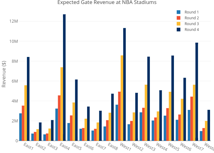
These equations will help us compute the expected gate revenue from any matchup between NBA teams with the two provided datasets. The expected gate revenue at NBA Stadiums is displayed below.

After running $1000$ playoff simulations (view code), we arrive at the following probability distribution:

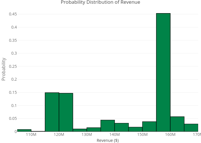
This distribution is bimodal, with the chance of generating $$160$ million or $$120$ million equal to about $75$%. If I were in the NBA Finance department, I would want to know which teams need to win in order to maximize playoff ticket sales. We can arrive at that answer by comparing which teams win at each round in simulations where the total revenue is $$160$ million and $$120$ million.

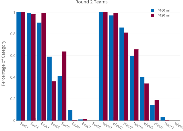
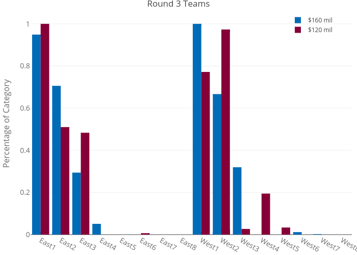
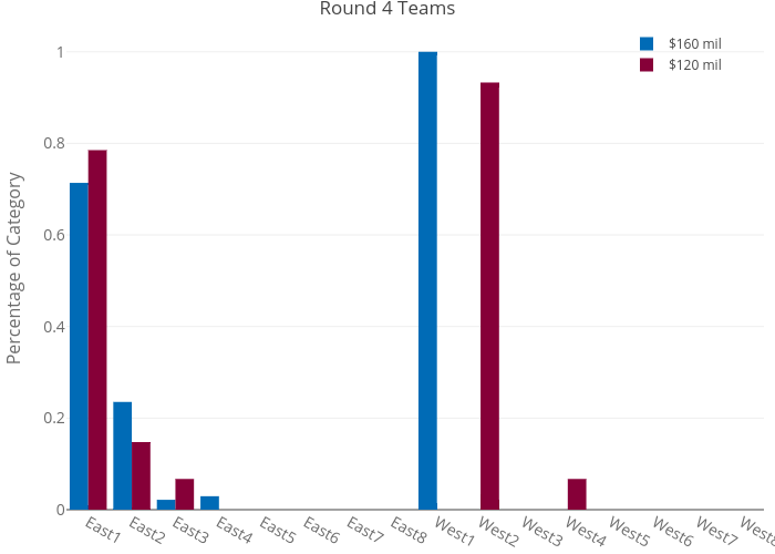
No huge discrepancies are present in the Round 2 and 3 plots, but the Round 4 plot, which shows us the NBA Finals participants, tells us everything we need to know: the top seed in the West (the 2017 Warriors), must make it to the Finals in order for the NBA to maximize their profit from ticket sales. Yes, most fans would suspect this to be true, but there’s nothing like proving intuitive suspicions with some math.