Dimensionality Reduction for Classification
Check out the Jupyter Notebook associated with this post!
The task of classification involves assigning every sample in a dataset to a specific category (or multiple categories), such as designating incoming emails as spam or not spam or labeling an image from the internet with its ImageNet category. An imbalanced dataset means that the classes are not represented equally by the data, such as a 75:1 ratio between mammograms of normal breast tissue and those containing cancerous tumors. A high-dimensional dataset means each sample contains many dimensions, such as mass spectrometry data or a large corpus of documents.
In this blog post, we will investigate how dimensionality reduction can facilitate the classification of a high-dimensional, imbalanced dataset. For tips and tricks specific to class imbalance, check out this blog post.
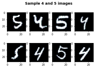
We will be working with a grayscale handwritten digits dataset, referred to as MNIST, which contains 55,0000 training images and 10,000 testing images and is a subset of a larger dataset produced by NIST. Each image is 28 x 28 or 784-dimensional. We will consider the task of classifying fours and fives but will only include 50 fives from the dataset to simulate class imbalance.
Dimensionality Reduction Techniques
Principal components analysis (PCA) relies upon the eigendecomposition of the centered covariance matrix, $S = YCY^T$, where $Y$ is the data matrix and $C$ is the centering matrix:
\[Y = V \lambda V^T\]PCA does not acknowledge possible correlation between the rows. The matrix $V$ of principal components can be used to transform data into the principle components. The sklearn implementation does not require the input data to be centered.
Singular Value Decomposition (SVD) essentially performs PCA on the columns and the rows of the data matrix and therefore takes into account possible correlation in the columns. SVD is commonly used in image analysis because the columns of an image matrix are usually correlated. In the SVD, the principal axis of variation of the columns of $Y$ are given by $U$, and the principal axis of variation of the rows of $Y$ are given by $V$:
\[Y = U \lambda^{1/2} V^T\]$V$ gives a description of column associations (within-row variation), and U gives
a description of row associations (within-column variation). The sklearn implementation performs this function but does not demean the input.
t-SNE is an extension of Stochastic Neighbor Embedding (SNE) that can produce non-linear 2D representations of high-dimensional datasets with much more latent structure than a linear technique like PCA. Consider high dimensional data points $X$ and their corresponding low dimensional embedding points $Y$. The SNE objective forces the distances between $Y$ to reflect those that exist in $X$. The conditional probability that a given point in $X$ would pick another point as its neighbor is given by:
\[p_{j | i} = \frac{\exp \left( - || x_i - x_j ||^2 / 2\sigma_i^2\right)}{\sum_{k \not = i}\exp \left( - || x_i - x_k ||^2 /2\sigma_i^2 \right) }\]The conditional probability that a given point in $Y$ would pick another point as its neighbor is given by:
\[q_{j | i} = \frac{\exp \left( - || y_i - y_j ||^2 \right)}{\sum_{k \not = i}\exp \left( - || y_i - y_k ||^2 \right) }\]The cost function to be minimized is the Kullback-Leibler divergence between $P_i$ and $Q_i$:
\[C = \sum_i KL(P_i || Q_i) = \sum_i \sum_j p_{j | i} \log \frac{p_{j | i}}{q_{j | i}}\]The cost function is minimized with gradient descent, and the gradient has a nice simple form:
\[\frac{\delta C}{\delta y_i} = 2 \sum (p_{j | i} - q_{j | i} + p_{i | j} - q_{i | j})(y_i - y_j)\]To determine the value of $\sigma_i$, SNE performs a binary search for that value that produces a $P_i$ with a fixed perplexity that is specified by the user: $ Perp(P_i) = 2^{H(P_i)} $, where $H(P_i)$ is the Shannon entropy of $P_i$ measured in bits: $ H(P_i) = -\sum_J p_{j | i} \log_2 p_{j |i } $. The perplexity can be interpreted as a smooth measure of the effective number of neighbors.
Several observations about SNE can be made:
- Each point $x_i$ has a unnormalized, scalable, multi-dimensional Gaussian around it. The Gaussian around points $y_i$ is not scalable.
- The probabilities are high for nearby points and almost $0$ for widely separated points.
- Since only pairwise similarities are of interest, $p_{i | i} = 0, q_{i | i} = 0$
- If the map points $y_i$ and $y_j$ correctly model the similarity between the high-dimensional data points. $x_i$ and $x_j$, the conditional probabilities $p_{j | i}$ and $q_{i | j}$ will be equal
- The KL cost function pushes distributions $P_i$ and $Q_i$ to be equal, but because KL is not symmetric, there is a large cost for using widely separated map points to represent nearby data points (i.e., for using a small $q_{j | i}$ to model a large $p_{j | i}$), but there is only a small cost for using nearby map points to represent widely separated data points.
t-SNE addresses two major drawbacks of SNE:
- SNE’s visualizations exhibited crowding at the center of the low dimensional space, so the Gaussian distribution on each point is replaced with a 1 degree t-distribution, which has approximate scale-invariance:
- SNE’s cost function was hard to optimize, so conditional probabilities are replaced by the joint probabilities, which yields a simpler gradient:
The sklearn implementation of t-SNE will yield different results each time, but this result is expected because t-SNE has a non-convex cost function.
Data Exploration and Classification
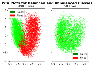
We can show that applying PCA to the entire dataset balanced with equal numbers of 4’s and 5’s yields good class separation; however, applying the same technique to the imbalanced dataset shows no separation.
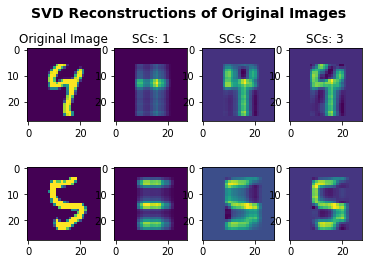
Applying SVD to individual images, unlike apply PCA to the entire dataset, yields discriminative features that we can use as the first step in our classification pipeline. Now we can represent each image as a vector of its concatenated singular components.
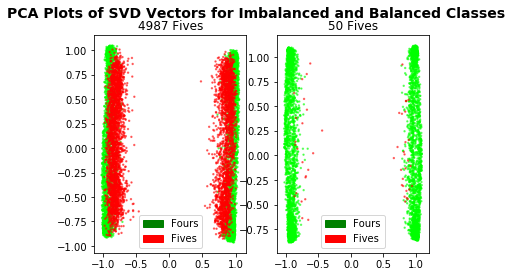
If we apply PCA to the matrix of the singular components, we get much better separation within the imbalanced dataset. Looking promising!
If we apply t-SNE to the SVD vectors, we see nice clustering of the fives. Feeding higher number of dimensions to the algorithm yields better separation.
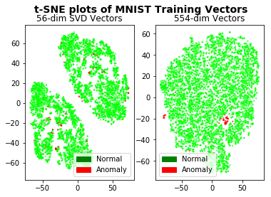
By tuning a threshold on the SVD vectors transformed by PCA, we can get an AUC of 0.902… not bad for a linear classifier!
Conclusion
Dimensionality reduction techniques can simply some binary classification problems to the point that only a linear classifier is needed to get a decent AUC, but for harder problems they can generate inputs to more complicated classifiers (i.e. neural networks and SVMs) that will improve the results. These techniques can also facilitate the exploration of class imbalanced datasets and the selection of the proper corrections. They should be the first line of defense against any challenging classification task!